MBB fits
Modified blackbody (MBB) fitting
Least squares fits
Observations of dust emission are often analysed by fitting the spectra with a modified blackbody function (MBB). This consists of the Planck law B(T) that is multiplied with a powerlaw, fβ. Here f stands for the observed frequency. By fitting multi-wavelength observations with this function, one can determine the temperature T of the dust particles (actually the “colour temperature” that is related to the temperature distribution within the telescope beam) and the spectral index β that should depend on the properties of the dust grains.
The MBB spectrum can be fitted to observations by finding the least squares solution (i.e. assuming that the measurements have normally distributed errors). When one is dealing with images, one takes the data for a single pixel (single spatial position), one value from each of the maps observed at different wavelengths, fits these with the MBB model, registers the resulting temperature and spectral index values – and moves to the next pixel. The only problem is that images may contain quite a few pixels, which can mean lengthy calculations. However, as long as one assumes that every pixel position can be fitted separately, that means that they can be computed in parallel.
We wrote a OpenCL program for the MBB fitting of dust observations and compared that to the use of scipy.optimize leastsq routine. The OpenCL algorithm is a very simple gradient descent method that in itself should be much less efficient that the least squares routines found in Scipy. However, the OpenCL version could have two advantages. First, the OpenCL is all compiled code, although we will be calling it from within a Python script. Also Scipy’s leastsq routine is a compiled library routine but it will call a function that is defined in Python and this will cause some overhead. Secondly, OpenCL routine will be run in parallel and especially on GPU with potentially thousands of concurrent threads.
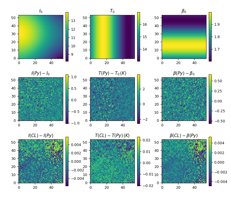
The first figure compares the results from the Python and OpenCL routines (using the default tolerances). The upper rows shows the intensity, temperature, and spectral index maps that were used to generate synthetic observations at 160, 250, 350, and 500µm wavelengths, to which we also added 3% of random errors. The second row shows the difference between the parameter values recovered by the Python least routine and the input values. The deviations from zero are almost entirely caused by the noise added to the observations. The last row shows the difference between the results from the OpenCL and the Python leastsq routines. With stricter tolerances the OpenCL solution approaches the leastsq solution. This suggests that the differences come mainly from the OpenCL solution. However, the accuracy already seems to be “good enough”, the difference between the OpenCL and Python solutions being two orders of magnitude smaller than the noise-induced uncertainty.
The next figure compares the run times between the Python leastsq solution and the OpenCL routine run on CPU and on two different GPUs. The analysed images ranged from 3×3 up to 1000×1000 pixels, the linear size of the image being on the x axis. Of course, only the total number of pixels matters and this varies by five orders of magnitude. On the y axis are the run times. Up to image sizes ~40×40, the Python routine is the fastest but all routines take less than one second to run. For larger images, the Python version is consistently some some ten times slower than the OpenCL routine that is run on the CPU. In addition to having four cores for parallel execution, the OpenCL routine has advantage from the use of compiled code that also seems to outweigh the effect of the efficient algorithm.
The most interesting result is the comparison between Python and the execution of the OpenCL routine on GPUs. When the image size approaches 1000×1000 pixels, the OpenCL routine is more than two orders of magnitude faster, even when run on the integrated GPU (GPU1 in the figure). On the more powerful external GPU, the OpenCL run time is still completely dominated by the constant overheads and remains close to one second! This is a good example of the potential of GPGPU computing. However, one should take into account that the example is one where Python is performing particularly poorly, because of the numerous calls to user-provided Python functions that are short and cannot make use of vector operations. MBB is also not a particularly difficult optimisation problem, especially since the range of acceptable temperature and spectra index values is rather limited. A general-purpose optimisation routine would be more complicated and probably also slower.