MAD
MAD -Median Absolute Deviation
MAD is calculated as the median of the absolute differences between data values and their median. For normal distribution MAD is equal to 1.48 times the standard deviation but is a more robust estimate of the dispersion of data values. The calculation of MAD is straightforward but time-consuming, especially if MAD estimates are needed for the local environment around every pixel of a large image. One such application was the Planck Galactic Cold Clumps Catalogue (PGCC, Planck Collaboration 2015 ) where the source detection pipeline used MAD values to estimate the reliability of the source detections (Montier et al. 2010 ). The all-sky Planck maps have of the order of 50 million pixels and thus MAD had to be calculated 50 million times (per detector band). In numerical simulations the number of pixels of a single synthetic map can easily be larger than this. If MAD is to be used, it must be fast.
In Python, MAD can be calculated using the generic_filter routine and a function
def fun(x):
    return np.median(np.abs(x-np.median(x)))
This is very concise. However, each call to the median function probably implies that the input vector is first sorted. In the initial tests with 4096×4096 pixel images, it took 16 minutes to calculate MAD estimates for every pixel location, using a filter size of 30 pixels across. Unfortunately, I had a project with 50 images of 8196×8196 pixels each. It would have taken more than two days to compute the corresponding MAD images.
Things could be improved by (1) improving the algorithm that computes MAD, by (2) replacing the Python routine with compiled code, (3) parallelising its execution, and (4) running on routine on GPU. After completing these steps, the run time of the previous example could be reduced from 946 seconds (16 minutes) down to 2.3 seconds. This is a speed-up of just over a factor of 400!
Part of the speed-up comes from an algorithm that does not sort the whole input array. Actually, the impact of this should be larger when MAD is computed for longer data vectors, instead of the 30-pixel radius areas (~100 pixels) in the example. The idea is that one first calculates the mean and standard deviation (one pass of the data), based on these sets up a number of bins (sub-intervals) and counts the number of data falling in each of the them (second pass). At this point one knows in which bin the median value falls. If the number of data points in that bin is still large, one can keep on subdividing the interval until the number of data points in the median-containing bin has fallen below some threshold. Finally, the data entries of that single bin are sorted and the median value is returned. In the test case, the total number of data points is similar to the selected number of sub-intervals. This means that once the data are divided into bins for the first time, the bin containing the median value is already likely to contain only a few data points. Therefore, one can directly proceed with the sorting, after having only twice passed through the full input data vector. The idea is similar to that of the [pigeonhole sort]{https://en.wikipedia.org/wiki/Pigeonhole_sort}, with the difference that to get the median value we do not need to sort the whole input vector, only the data in the bin containing the median. The method was implemented OpenCL and the pyopencl library, Therefore, we can call the OpenCL routine directly from Python programs.
The next figure shows another comparison of the run time between the Python scipy solution (as mentioned above) and the OpenCL routine run on CPU and on GPU. The size of the analysed image is varied from 32×32 up to 10000×10000 pixels, as indicated by the x axis. The filter is here square and 11×11 pixels in size.

The scipy version is fastest only for the smallest 32×32 pixel images. For large images the OpenCL version is on CPU some 35 times faster – and still much faster son GPU. For 1000×1000 pixel images, the GPU is a factor of 800 faster than the original scipy routine and some 20 times faster than the OpenCL routine on CPU. While the scipy and OpenCL/CPU solutions show a similar scaling, the relative advantage of the GPU is still increasing for the largest maps.
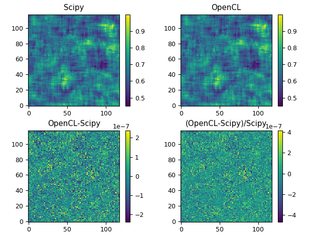
The last image below contains a comparison between the results of the scipy and OpenCL routines, which shows that the results are indeed almost identical. The upper frames show the filtered images when the inputs are generated with normally distributed random numbers as max(1.0,2.0+N(0,1)). The lower frames show the difference between the results as absolute and relative differences.
