Filaments

Filaments

Filaments appear to be an important structural component of the interstellar medium (ISM) and closely connected to the star formation. ISM studies need tools that automatise the finding of filamentary structures and the estimation of their properties.

Filament extraction

In the paper Juvela (2016) the template matching was already suggested as a fast way to locate (among other things) elongated structures from images (see template matching ). The goodness of the match between the template and the image structures was based on the straight sum of the product of the template and the image pixels at the locations of the template elements (for the location and position angle of the template). With small changes this can be converted an algorithm that estimates the actual probability of a pixel belonging to a filament.

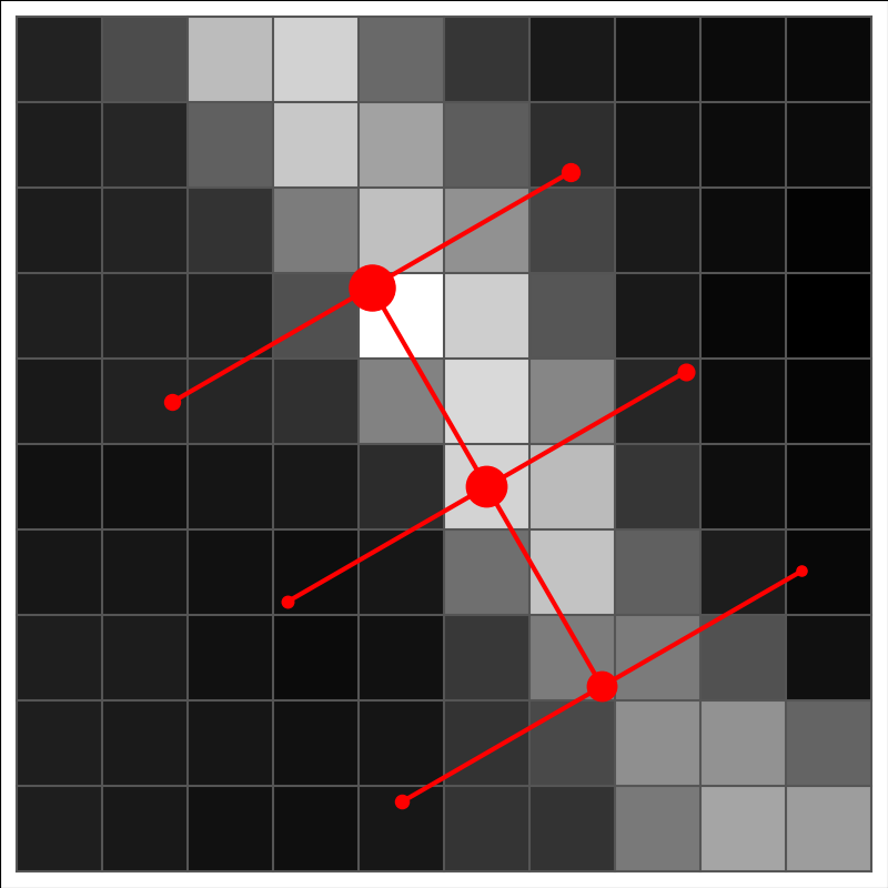
We start again with a 3×3 element pattern that forms a square with a fixed step between the elements. Instead of assigning fixed values for the elements (as in the case of template matching), we simply place the pattern on the image, at the position of each image pixel and with different position angles. For each position and position angle, we calculate the probability of this corresponding to an actual filament crossing the current image location, in the current tested direction. The probability is based on a simple definition of a filament: in the filament direction, the pixel values matching the central line of the 3×3 element pattern should be higher than either of the pixel values on the left and right hand sides of that line. To compute this probability, one must first calculate the standard deviation for the change of the pixel values at the scale of step. This takes into account that one is likely to operate close to the spatial resolution of the images and the pixels at the separation of the distance step can be partially correlated.

The above figure shows a stencil (nine red points) on an image. The step between the stencil points is not tied to the pixelisation. However, the step parameter (distance between the stencil elements) defines the scale at which the filaments are most likely to be extracted. This could be combined with preprocessing where the input map is first convolved (to remove small-scale structure when one is only interested in structures at larger scales) or also high-pass filtered (to reduced the effect of larger, e.g. gradients than the intended width of the filaments (e.g. gradients).

The first step of the analysis results in two maps, one for the filament probability and one for the most likely position angle. The dimensions of these maps are the same as that of the input map. In the second step, the probability map is thresholded. The pixels above the threshold are divided into connected regions and they are numbered sequentially as potential filaments. The final part of the analysis is the tracing of the filaments. This gives a list of coordinates describing the spine of each filament and enables one to extract an image of each individual filament (one coordinate running along the filament and one perpendicular to the filament). As one traces the filament, one may also want to update the probability estimates that were computed only locally. Our trust in a weak detection should be strengthened if the filament is seen to continue in either direction (with a matching position angle).

The program ocfil implements the above ideas, using OpenCL to parallelise the operations. The initial calculation of per-pixel probabilities is very fast, even when the calculation needs to be done for tens of thousands of pixels, in each case testing at least ~10 position angles. After probability thresholding, the image segmentation is done with the scipy.ndimage routines label(). Finally, separate OpenCL kernels are used to trace the filaments and to extract their images.

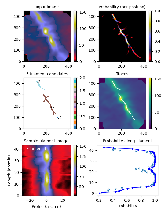
The above figure shows the results for the Herschel 250µm map of the Musca filament, for an image convolved to one arcmin resolution and using step equal to one arcmin. The frames correspond to the analysis steps: (1) convolved input map, (2) estimated per-pixel probabilities (position angles not shown), (3) thresholding giving the pixels belonging to each filament, (4) traced filament skeletons, (5) extraction of the 2d image of an filament (here only the longest filament shown), and (6) the estimated “filament probability” along the filament. In the last frame, the open circles for the original probability while the solid line takes into account some evidence from the filament continuity.

For this map of ~200 000 pixels, the run time was below one second (on a GPU, including the plotting). For large maps there may still be some bottlenecks. The processing of a 8192×8192 image of an MHD simulation resulted in the detection of close to 13000 filaments, in calculations that took some ten seconds. However, this timing did not include the final step, the tracing of the filament skeletons.

The main advantages of the code are the simple, non-black-box definition of filaments (one that also matches well the extraction by eye), fast run times, and the small amount of code. There are some 200 lines of code in the OpenCL kernel, 200 lines in the Python main program, with few additional ancillary routines. While the probability calculations and image segmentation are straightforward, the tracing of the filaments will need more work. For example, the initial filament tracing routine did not handle branching filaments, as also shown by the above figure. The files on GitHub include two alternative methods that try to address this point.

The code for ocfil can be found at GitHub , in the OCFIL subdirectory.